Bank Customers’ Churn Prediction
Abdullah Albyati
Business School, Golden Gate University
MSBA 307: AI for Data Security, Integrity and Risk Mitigation
November 28, 2021
Table of Contents
Problem Statement
The credit card services division of XYZ bank is experiencing customers closing their accounts. The current churn rate is 16.07%. Because the cost of retaining an existing customer is far less than acquiring a new one, the bank is looking to predict which customers might get churned so they can proactively go to the customer to provide them with better services.
Proposed Solution

In this analysis, I will work through the steps of the proposed solution. The ideal solution should provide the business with and accurate estimates of potential customers who are at risk of churn. Before I dig deeper into the solution and the implementation let’s explore what is the churn rate, why it is important, and its impact on the business.
Churn rate, also known as attrition rate and is the rate at which, customers stop doing business with the bank, or close their account (source).
In this analysis, two models were implemented and can be used together or separately by the bank to understand how to better manage their churn rate.
The first model is cluster analysis, cluster analysis is used to group the bank’s customers into groups of similar characteristics (source) these groups can then be used to identify which cluster has the highest amount of churned customers then look at that cluster to build the at-risk customer profile.
The second model is a binary classification model, where the data is used to predict whether the customer will churn or not. A binary classification model takes labeled data and assigns it to a category in our analysis the model will assign churned customers to 1 and existing customers to 0.
Data Source
The data and the problem to solve is retrieved from a Kaggle repository
Importing Libraries
import numpy as np
import pandas as pd
import matplotlib.pyplot as plt
import seaborn as sns
import plotly
import plotly.express as px
from sklearn.model_selection import train_test_split
from sklearn.preprocessing import MinMaxScaler
import plotly.io as pio
from sklearn.tree import DecisionTreeClassifier
from sklearn.ensemble import RandomForestClassifier, GradientBoostingClassifier, AdaBoostClassifier
from sklearn.metrics import recall_score
#pio.renderers.default='notebook'
pd.options.plotting.backend = "plotly"
from matplotlib.pyplot import figure
from dataprep.eda import plot, plot_correlation, plot_missing
plotly.offline.init_notebook_mode(connected=True)
import warnings
warnings.filterwarnings('ignore')
Exploratory Data Analysis
To explore the data set and conduct an initial analysis, python’s dataprep.EDA package will be used. This package is the most efficient way to take a quick look at the data summary statistics and plot all variables of the data in one command.
# import the data to the workbook
df = pd.read_csv('BankChurners.csv')
df = df.iloc[:,1:-2] # remove ID column and last 2 columns
# use dataprep plot function to generate an EDA report
plot(df, config={'height': 200, 'width': 300, })
| Number of Variables | 20 |
|---|---|
| Number of Rows | 10127 |
| Missing Cells | 0 |
| Missing Cells (%) | 0.0% |
| Duplicate Rows | 0 |
| Duplicate Rows (%) | 0.0% |
| Total Size in Memory | 4.9 MB |
| Average Row Size in Memory | 503.2 B |
| Variable Types |
|
| Months_on_book is skewed | Skewed |
|---|---|
| Credit_Limit is skewed | Skewed |
| Total_Revolving_Bal is skewed | Skewed |
| Avg_Open_To_Buy is skewed | Skewed |
| Total_Amt_Chng_Q4_Q1 is skewed | Skewed |
| Total_Ct_Chng_Q4_Q1 is skewed | Skewed |
| Avg_Utilization_Ratio is skewed | Skewed |
| Attrition_Flag has constant length 17 | Constant Length |
| Gender has constant length 1 | Constant Length |
| Dependent_count has constant length 1 | Constant Length |
| Total_Relationship_Count has constant length 1 | Constant Length |
|---|---|
| Months_Inactive_12_mon has constant length 1 | Constant Length |
| Contacts_Count_12_mon has constant length 1 | Constant Length |
| Total_Revolving_Bal has 2470 (24.39%) zeros | Zeros |
| Avg_Utilization_Ratio has 2470 (24.39%) zeros | Zeros |
- 1
- 2
As the summary statistics show we have 20 total variables (Categorical: 10, Numerical: 10), a total of 10127 rows with 0 missing data. The Attrition_Flag plot also shows that 84% of the data is of existing customers and 16% of attrited/churned customers which means the data set is imbalanced. An imbalanced dataset is where data is disproportionate dispersed where there is a higher ratio of observations in a specific class (source). Since the data is imbalanced a careful model metric and model evaluation scoring were selected (see models for more info)
Data Cleaning and Preparation
For the data to be ready for a machine learning model the data column types should be either numeric or categorical data, below we will clean the data by changing some column types manually like the attrition flag column, and in some other columns we will use the one-hot encoding method
# Change flag to numerical
df["Attrition_Flag"] = df["Attrition_Flag"].map({"Existing Customer":0, "Attrited Customer":1})
# convert columns of type object to categorical columns
cols=df.select_dtypes(exclude=['int64', 'float64']).columns.to_list()
df[cols]=df[cols].astype('category')
df.info()
<class 'pandas.core.frame.DataFrame'> RangeIndex: 10127 entries, 0 to 10126 Data columns (total 20 columns): # Column Non-Null Count Dtype --- ------ -------------- ----- 0 Attrition_Flag 10127 non-null int64 1 Customer_Age 10127 non-null int64 2 Gender 10127 non-null category 3 Dependent_count 10127 non-null int64 4 Education_Level 10127 non-null category 5 Marital_Status 10127 non-null category 6 Income_Category 10127 non-null category 7 Card_Category 10127 non-null category 8 Months_on_book 10127 non-null int64 9 Total_Relationship_Count 10127 non-null int64 10 Months_Inactive_12_mon 10127 non-null int64 11 Contacts_Count_12_mon 10127 non-null int64 12 Credit_Limit 10127 non-null float64 13 Total_Revolving_Bal 10127 non-null int64 14 Avg_Open_To_Buy 10127 non-null float64 15 Total_Amt_Chng_Q4_Q1 10127 non-null float64 16 Total_Trans_Amt 10127 non-null int64 17 Total_Trans_Ct 10127 non-null int64 18 Total_Ct_Chng_Q4_Q1 10127 non-null float64 19 Avg_Utilization_Ratio 10127 non-null float64 dtypes: category(5), float64(5), int64(10) memory usage: 1.2 MB
Now the data contains only numerical and categorical data and we can do Hot Encoding on it below
Hot Encoding
One-hot encoding creates new columns indicating the presence (or absence) of each possible value in the original data. To understand this, we'll work through an example.
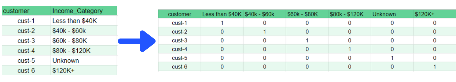
In the original dataset, "Income_Category" is a categorical variable with six variables: Less than $40K, $40k - $60k, $60k - $80K, $80k - $120K, Unknown, $120K+. The corresponding one-hot encoding contains one column for each possible value and one row for each row in the original dataset. Wherever the original value was "Less than $40K", we put a 1 in the "Less than $40K" column; if the original value was "$80k - $120K", we put a 1 in the "$80k - $120K" column, and so on. One-hot encoding generally does not perform well if the categorical variable takes on a large number of values (i.e., you generally won't use it for variables taking more than 15 different values). source
# Credit to https://stackoverflow.com/questions/37292872/how-can-i-one-hot-encode-in-python
def encode_and_bind(original_dataframe, feature_to_encode):
dummies = pd.get_dummies(original_dataframe[[feature_to_encode]])
res = pd.concat([original_dataframe, dummies], axis=1)
res = res.drop([feature_to_encode], axis=1)
return(res)
features_to_encode = df.select_dtypes('category').columns.to_list()
for feature in features_to_encode:
df = encode_and_bind(df, feature)
df.info()
<class 'pandas.core.frame.DataFrame'> RangeIndex: 10127 entries, 0 to 10126 Data columns (total 38 columns): # Column Non-Null Count Dtype --- ------ -------------- ----- 0 Attrition_Flag 10127 non-null int64 1 Customer_Age 10127 non-null int64 2 Dependent_count 10127 non-null int64 3 Months_on_book 10127 non-null int64 4 Total_Relationship_Count 10127 non-null int64 5 Months_Inactive_12_mon 10127 non-null int64 6 Contacts_Count_12_mon 10127 non-null int64 7 Credit_Limit 10127 non-null float64 8 Total_Revolving_Bal 10127 non-null int64 9 Avg_Open_To_Buy 10127 non-null float64 10 Total_Amt_Chng_Q4_Q1 10127 non-null float64 11 Total_Trans_Amt 10127 non-null int64 12 Total_Trans_Ct 10127 non-null int64 13 Total_Ct_Chng_Q4_Q1 10127 non-null float64 14 Avg_Utilization_Ratio 10127 non-null float64 15 Gender_F 10127 non-null uint8 16 Gender_M 10127 non-null uint8 17 Education_Level_College 10127 non-null uint8 18 Education_Level_Doctorate 10127 non-null uint8 19 Education_Level_Graduate 10127 non-null uint8 20 Education_Level_High School 10127 non-null uint8 21 Education_Level_Post-Graduate 10127 non-null uint8 22 Education_Level_Uneducated 10127 non-null uint8 23 Education_Level_Unknown 10127 non-null uint8 24 Marital_Status_Divorced 10127 non-null uint8 25 Marital_Status_Married 10127 non-null uint8 26 Marital_Status_Single 10127 non-null uint8 27 Marital_Status_Unknown 10127 non-null uint8 28 Income_Category_$120K + 10127 non-null uint8 29 Income_Category_$40K - $60K 10127 non-null uint8 30 Income_Category_$60K - $80K 10127 non-null uint8 31 Income_Category_$80K - $120K 10127 non-null uint8 32 Income_Category_Less than $40K 10127 non-null uint8 33 Income_Category_Unknown 10127 non-null uint8 34 Card_Category_Blue 10127 non-null uint8 35 Card_Category_Gold 10127 non-null uint8 36 Card_Category_Platinum 10127 non-null uint8 37 Card_Category_Silver 10127 non-null uint8 dtypes: float64(5), int64(10), uint8(23) memory usage: 1.4 MB
Correlation Analysis
Correlation shows the relationship between 2 variables and how each variable affects the other. A positive correlation explains as 1 variable increases the other related variables also increase. A negative correlation is the opposite as an increase in one variable causes a decrease in another (source)
Negative Correlation
plot_correlation(df, "Attrition_Flag", value_range=[-1, - 0.01])
The correlation heatmap above shows any features in our dataset that have a negative correlation with the attrition flag. We can see that the total transaction count has the highest negative correlation of -0.37 which means the lower the number of transactions the customer has the more likely for them to cancel their account. All other columns that have a negative correlation with the attrition flag can be translated similarly
Positive Correlation
plot_correlation(df, "Attrition_Flag", value_range=[0.01, 1])
The correlation heatmap above shows any features in our dataset that have a positive correlation with the attrition flag. We can see that the months inactive and contact count has the highest correlation with the attrition flag at 0.20 and 0.15 respectively which means the higher the months inactive and the numbers of contact the more likely for the customer to cancel their account.
Machine Learning Model
Clustering
As mentioned earlier cluster analysis is used to group the bank’s customers into groups of similar characteristics (source) these groups can then be used to identify which cluster has the highest amount of churned customers then look at that cluster to build the at-risk customer profile. For this analysis, I will use K-means clustering due to its simplicity, precision, and low number of parameters to tune, K-means is an unsupervised machine learning algorithm that takes a set of data and assigns the data to a specific number of clusters. K-means selects a random center for each cluster and assigns the closest points to that center to the cluster.
To determine the optimal number of clusters for the dataset we utilize the elbow method We graph the relationship between the number of clusters and the Cluster Sum of Squares (WCSS) which is the sum of the squared distance between each member of the cluster and its centroid. then we select the number of clusters where the change in WCSS begins to level off (source), in our case the value is 4 as the chart below shows.
from sklearn.cluster import KMeans
wcss = []
for k in range(1,11):
kmeans = KMeans(n_clusters=k, init="k-means++")
kmeans.fit(df)
wcss.append(kmeans.inertia_)
plt.figure(figsize=(12,6))
plt.grid()
plt.plot(range(1,11),wcss, linewidth=2, color="red", marker ="8")
plt.xlabel("K Value")
plt.xticks(np.arange(1,11,1))
plt.ylabel("WCSS")
plt.show()

Now we have the optimal number of clusters we use it to build the clustering model which return the following
kmeans = KMeans(n_clusters=4, init='k-means++', max_iter=300, n_init=10, random_state=0)
clusters = kmeans.fit_predict(df)
df_culstered = df
df_culstered["cluster"] = clusters
sns.set(style="whitegrid")
plt.figure(figsize=(10,8))
total = float(len(df))
ax = sns.countplot(x="cluster", hue="Attrition_Flag", data=df_culstered)
plt.title('Clusters By Attrition', fontsize=20)
for p in ax.patches:
percentage = '{:.1f}%'.format(100 * p.get_height()/total)
x = p.get_x() + p.get_width()
y = p.get_height()+2
ax.annotate(percentage, (x, y),ha='center')
plt.show()

As we can see from the chart above the majority of the customers that closed their account falls in cluster 0. The alarming trend is that majority of the bank customers are in cluster 0 and these customers are at risk and will require immediate proactive reach to ensure the customers stay with the bank. Now let’s plot cluster 0 population and understand the cluster profile
cluster_0 = df_culstered.query('cluster == 0 & Attrition_Flag == 1')
plot(cluster_0, config={'height': 200, 'width': 300, })
| Number of Variables | 39 |
|---|---|
| Number of Rows | 1013 |
| Missing Cells | 0 |
| Missing Cells (%) | 0.0% |
| Duplicate Rows | 0 |
| Duplicate Rows (%) | 0.0% |
| Total Size in Memory | 153.3 KB |
| Average Row Size in Memory | 155.0 B |
| Variable Types |
|
| Months_on_book is skewed | Skewed |
|---|---|
| Credit_Limit is skewed | Skewed |
| Total_Revolving_Bal is skewed | Skewed |
| Avg_Open_To_Buy is skewed | Skewed |
| Total_Trans_Amt is skewed | Skewed |
| Total_Trans_Ct is skewed | Skewed |
| Avg_Utilization_Ratio is skewed | Skewed |
| Attrition_Flag has constant value "1" | Constant |
| Card_Category_Gold has constant value "0" | Constant |
| Card_Category_Platinum has constant value "0" | Constant |
| cluster has constant value "0" | Constant |
|---|---|
| Attrition_Flag has constant length 1 | Constant Length |
| Dependent_count has constant length 1 | Constant Length |
| Total_Relationship_Count has constant length 1 | Constant Length |
| Months_Inactive_12_mon has constant length 1 | Constant Length |
| Contacts_Count_12_mon has constant length 1 | Constant Length |
| Gender_F has constant length 1 | Constant Length |
| Gender_M has constant length 1 | Constant Length |
| Education_Level_College has constant length 1 | Constant Length |
| Education_Level_Doctorate has constant length 1 | Constant Length |
| Education_Level_Graduate has constant length 1 | Constant Length |
|---|---|
| Education_Level_High School has constant length 1 | Constant Length |
| Education_Level_Post-Graduate has constant length 1 | Constant Length |
| Education_Level_Uneducated has constant length 1 | Constant Length |
| Education_Level_Unknown has constant length 1 | Constant Length |
| Marital_Status_Divorced has constant length 1 | Constant Length |
| Marital_Status_Married has constant length 1 | Constant Length |
| Marital_Status_Single has constant length 1 | Constant Length |
| Marital_Status_Unknown has constant length 1 | Constant Length |
| Income_Category_$120K + has constant length 1 | Constant Length |
| Income_Category_$40K - $60K has constant length 1 | Constant Length |
|---|---|
| Income_Category_$60K - $80K has constant length 1 | Constant Length |
| Income_Category_$80K - $120K has constant length 1 | Constant Length |
| Income_Category_Less than $40K has constant length 1 | Constant Length |
| Income_Category_Unknown has constant length 1 | Constant Length |
| Card_Category_Blue has constant length 1 | Constant Length |
| Card_Category_Gold has constant length 1 | Constant Length |
| Card_Category_Platinum has constant length 1 | Constant Length |
| Card_Category_Silver has constant length 1 | Constant Length |
| cluster has constant length 1 | Constant Length |
| Total_Revolving_Bal has 557 (54.99%) zeros | Zeros |
|---|---|
| Avg_Utilization_Ratio has 557 (54.99%) zeros | Zeros |
- 1
- 2
- 3
- 4
- 5
Attrited Customer Profile
- 85% of customers in this cluster have had more than 1 support call in the last 12 months
- Low credit limit between 2000 and 7000 with the majority of customers at the lower end of this range.
- Inactive months between 2 and 4 months for the majority of this cluster.
- 0 revolving balance, the majority of attrited customers in this cluster have 0 revolving balance.
- 75% of customers in this cluster are Females
- Lower-income category, less than $40K
- Blue card category
Classification Model
The dataset contains 84% existing customers and only 16% attired customers so the data is imbalanced and in order to test a classification model for accuracy the Matthews Correlation Coefficient (MCC) is selected. MCC metric does better in scoring classification models with imbalanced data (source)
Now we split our dataset into training data and prediction data and score it across 5 different classification models and select the best model.
from sklearn.metrics import matthews_corrcoef
from sklearn.linear_model import LogisticRegression
from sklearn.ensemble import GradientBoostingClassifier
from sklearn.ensemble import AdaBoostClassifier
from sklearn.ensemble import RandomForestClassifier
from xgboost import XGBClassifier
X = df.loc[:, ~df.columns.isin(['Attrition_Flag', 'cluster'])]
y = df["Attrition_Flag"].astype("uint8")
X_train, X_test, y_train, y_test = train_test_split(X, y, test_size = 0.25,random_state=1)
# the models to test
models = []
models.append(("LogisticRegression", LogisticRegression(random_state=1)))
models.append(("GradientBoostingClassifier", GradientBoostingClassifier(random_state=1)))
models.append(("AdaBoostClassifier", AdaBoostClassifier(random_state=1)))
models.append(("XGBClassifier",XGBClassifier(random_state=1, verbosity = 0)))
models.append(("RandomForestClassifier", RandomForestClassifier(random_state=1)))
# evaluate each model in turn
MCC_score = []
names = []
for name, model in models:
model.fit(X_train, y_train)
pred = model.predict(X_test)
MCC = matthews_corrcoef(y_test, pred)
MCC_score.append(MCC)
names.append(name)
scored = pd.DataFrame(zip(names, MCC_score),
columns=["model", "MCC_Score"])
scored
| model | MCC_Score | |
|---|---|---|
| 0 | LogisticRegression | 0.482800 |
| 1 | GradientBoostingClassifier | 0.868394 |
| 2 | AdaBoostClassifier | 0.829310 |
| 3 | XGBClassifier | 0.893396 |
| 4 | RandomForestClassifier | 0.824039 |
The XGBClassifier model scored the highest score and therefore I will use it to build the model and the prediction. Before I continue further below is some background explaining the XGBClassifier. The XGBClassifier is a classification model from the XGBoost library which is an optimized distributed gradient boosting library designed to be highly efficient, flexible, and portable. It implements machine learning algorithms under the Gradient Boosting framework (source). XGBoost is short for “eXtreme Gradient Boosting.” The “eXtreme” refers to speed enhancements that make XGBoost approximately 10 times faster than traditional Gradient Boosting like the random forest algorithm uses.
Now we have our model selected we will train the model, create predictions and see the model metrics. The model is evaluated using the confusion matrix and its corresponding matrics. A confusion matrix is a table of
- True Positive (TP): a value of 1 that was correctly classified as 1, in our case, this means an attrited customer correctly classified as an attrited customer.
- False Positive(FP): a value of 1 that was incorrectly classified as 0, in our case, this means an attrited customer was incorrectly classified as an existing customer.
- False Negative(FN): a value of 0 that was incorrectly classified as 1, in our case, this means an existing customer was incorrectly classified as an attrited customer.
- True Negative(TN): a value of 0 that was correctly classified as 0, in our case, this means an existing customer was correctly classified as an existing customer.
For our analysis, our focus is to accurately predict the True Positive cases which is an attrited customer classification. Having the confusion matrix help us calculate the following metrics:
Accuracy: The ratio of correct prediction to the total prediction
Precision: The number of classes correctly classified divided by the number of predictions.
Recall: The ratio of total numbers correctly flagged attrited customers to the total number of attrited customers. This metric is the most important for our use case as it measures the success of the attrited customers.
Initial Model Performance
from sklearn.metrics import confusion_matrix, plot_confusion_matrix, accuracy_score, precision_score, recall_score
xgb_model = XGBClassifier(random_state=1)
xgb_model.fit(X_train, y_train)
cfm = confusion_matrix(y_true=y_test, y_pred=xgb_model.predict(X_test))
y_pred = xgb_model.predict(X_test)
TN, FP, FN, TP = cfm.ravel()
fig, ax = plt.subplots(figsize=(12, 8))
group_names = ["True Neg","False Pos", "False Neg", "True Pos"]
group_counts = ["{0:0.0f}".format(value) for value in
cfm.flatten()]
labels = [f"{v1}\n{v2}" for v1, v2 in
zip(group_names,group_counts)]
labels = np.asarray(labels).reshape(2,2)
ax = sns.heatmap(cfm, annot=labels, fmt="", cmap='Blues')
plt.title('Model Confusion Matrix', fontsize = 20) # title with fontsize 20
plt.xlabel('Actual', fontsize = 15) # x-axis label with fontsize 15
plt.ylabel('Predicted', fontsize = 15) # y-axis label with fontsize 15
print("*" * 30)
print("Accuracy :", accuracy_score(y_true=y_test, y_pred=xgb_model.predict(X_test)))
print("Precision :", precision_score(y_true=y_test, y_pred=xgb_model.predict(X_test)))
print("Recall :", recall_score(y_true=y_test, y_pred=xgb_model.predict(X_test)))
print("*" * 30)
plt.show()
****************************** Accuracy : 0.9715639810426541 Precision : 0.9193954659949622 Recall : 0.9012345679012346 ******************************

Model Tunning
Important Features Selection
After the one-hot encoding method described above the dataset now have 37 total features used in the initial model. It is important to note that sometimes having too many features in the model affects the model accuracy as some features affect the prediction and it can slow the model tremendously. With that in mind, I will use the python library Scikit-Learn feature selection via SelectFromModel which selects the best features based on the importance of these features on a specific metric. The code below runs through our model features and change the features used in the prediction and compares the recall score every time and gives us the features used for a model that had a recall score higher than the initial model recall score
from numpy import loadtxt
from numpy import sort
from xgboost import XGBClassifier
from sklearn.model_selection import train_test_split
from sklearn.metrics import accuracy_score
from sklearn.feature_selection import SelectFromModel
X = df.loc[:, ~df.columns.isin(['Attrition_Flag', 'cluster'])]
y = df["Attrition_Flag"].astype("uint8")
X_train, X_test, y_train, y_test = train_test_split(X, y, test_size = 0.25,random_state=1)
feature_names = np.asarray(list(X.columns))
model = XGBClassifier(random_state=1)
model.fit(X_train, y_train)
# make predictions for test data and evaluate
predictions = model.predict(X_test)
Recall = recall_score(y_test, predictions)
print("Initial Recall: %.2f%%" % (Recall * 100.0))
# Fit model using each importance as a threshold
thresholds = sort(model.feature_importances_)
for thresh in thresholds:
# select features using threshold
selection = SelectFromModel(model, threshold=thresh, prefit=True)
select_X_train = selection.transform(X_train)
# train model
selection_model = XGBClassifier(random_state=1)
selection_model.fit(select_X_train, y_train)
# eval model
select_X_test = selection.transform(X_test)
selected_features = feature_names[selection.get_support()]
predictions = selection_model.predict(select_X_test)
accuracy = recall_score(y_test, predictions)
if accuracy > Recall:
print("Thresh=%.3f, n=%d, New Recall: %.2f%%, Features selected by SelectFromModel: %s" % (thresh, select_X_train.shape[1], accuracy*100.0, selected_features))
Initial Recall: 90.12% Thresh=0.018, n=14, New Recall: 90.37%, Features selected by SelectFromModel: ['Customer_Age' 'Total_Relationship_Count' 'Months_Inactive_12_mon' 'Contacts_Count_12_mon' 'Credit_Limit' 'Total_Revolving_Bal' 'Avg_Open_To_Buy' 'Total_Amt_Chng_Q4_Q1' 'Total_Trans_Amt' 'Total_Trans_Ct' 'Total_Ct_Chng_Q4_Q1' 'Gender_F' 'Marital_Status_Married' 'Card_Category_Blue'] Thresh=0.026, n=10, New Recall: 90.37%, Features selected by SelectFromModel: ['Customer_Age' 'Total_Relationship_Count' 'Months_Inactive_12_mon' 'Total_Revolving_Bal' 'Avg_Open_To_Buy' 'Total_Amt_Chng_Q4_Q1' 'Total_Trans_Amt' 'Total_Trans_Ct' 'Total_Ct_Chng_Q4_Q1' 'Marital_Status_Married']
Now we use these features to recalculate the model metrics and confusion matrix to see if the model has improved.
X = df[['Customer_Age', 'Total_Relationship_Count', 'Months_Inactive_12_mon',
'Contacts_Count_12_mon', 'Credit_Limit', 'Total_Revolving_Bal',
'Avg_Open_To_Buy', 'Total_Amt_Chng_Q4_Q1', 'Total_Trans_Amt',
'Total_Trans_Ct', 'Total_Ct_Chng_Q4_Q1', 'Gender_F',
'Marital_Status_Married', 'Card_Category_Blue']]
y = df["Attrition_Flag"].astype("uint8")
X_train, X_test, y_train, y_test = train_test_split(X, y, test_size = 0.25,random_state=1)
xgb_model = XGBClassifier(random_state=1)
xgb_model.fit(X_train, y_train)
cfm = confusion_matrix(y_true=y_test, y_pred=xgb_model.predict(X_test))
y_pred = xgb_model.predict(X_test)
TN, FP, FN, TP = cfm.ravel()
fig, ax = plt.subplots(figsize=(12, 8))
group_names = ["True Neg","False Pos", "False Neg", "True Pos"]
group_counts = ["{0:0.0f}".format(value) for value in
cfm.flatten()]
labels = [f"{v1}\n{v2}" for v1, v2 in
zip(group_names,group_counts)]
labels = np.asarray(labels).reshape(2,2)
sns.heatmap(cfm, annot=labels, fmt="", cmap='Blues')
plt.title('Model Confusion Matrix', fontsize = 20) # title with fontsize 20
plt.xlabel('Actual', fontsize = 15) # x-axis label with fontsize 15
plt.ylabel('Predicted', fontsize = 15) # y-axis label with fontsize 15
print("*" * 30)
print("Accuracy :", accuracy_score(y_true=y_test, y_pred=y_pred))
print("Precision :", precision_score(y_true=y_test, y_pred=y_pred))
print("Recall :", recall_score(y_true=y_test, y_pred=y_pred))
print("*" * 30)
****************************** Accuracy : 0.9747235387045814 Precision : 0.9360613810741688 Recall : 0.9037037037037037 ******************************

Hyper Parameters Tunning
Parameters tunning is an approach to adjusting the model parameters to improve the model accuracy, this technique can be very time-consuming and requires high computation especially in the case of models with many parameters like the model we are using.
The XGBClassifier model has 31 total parameters (see documentation%20%E2%80%93-,class,%EF%83%81,-Bases%3A%20xgboost.sklearn.XGBModel%2C%20object)) and adjusting all of them will not be possible without high computing power. We will attempt to tune the following parameters as they are considered important to model performance and accuracy (Source)
learning_rate: used to avoid model overfitting in Gradient boosting models
n_estimators: Gradient boosting involves the creation and addition of decision trees sequentially, each attempting to correct the mistakes of the learners that came before it. This parameter adjusts the number of trees in the model. (Source)
max_depth: The depth of each tree from the n_estimators parameter.
To adjust these parameters and see if the model improves the GridSearchCV a scikit-learn’s hyperparameter tuning function which takes a list of parameters and re-run the model with all possible combinations of the parameters and score each output against a chosen metric.
from sklearn.preprocessing import LabelBinarizer
from sklearn.ensemble import RandomForestClassifier
from sklearn.model_selection import train_test_split, GridSearchCV, StratifiedKFold
from sklearn.metrics import roc_curve, precision_recall_curve, auc, make_scorer, recall_score, accuracy_score, precision_score, confusion_matrix
X = df[['Customer_Age', 'Total_Relationship_Count', 'Months_Inactive_12_mon',
'Contacts_Count_12_mon', 'Credit_Limit', 'Total_Revolving_Bal',
'Avg_Open_To_Buy', 'Total_Amt_Chng_Q4_Q1', 'Total_Trans_Amt',
'Total_Trans_Ct', 'Total_Ct_Chng_Q4_Q1', 'Gender_F',
'Marital_Status_Married', 'Card_Category_Blue']]
y = df["Attrition_Flag"].astype("uint8")
X_train, X_test, y_train, y_test = train_test_split(X, y, test_size = 0.25,random_state=1)
clf = XGBClassifier(random_state=1)
param_grid = {
"learning_rate": [0.0001, 0.001, 0.01, 0.1, 0.2, 0.3],
"n_estimators": [100, 200, 300, 400, 500],
"random_state": [1],
"max_depth": [3,4,5,6,7]
}
scorers = {
'precision_score': make_scorer(precision_score),
'recall_score': make_scorer(recall_score),
'accuracy_score': make_scorer(accuracy_score)
}
def grid_search_wrapper(refit_score='precision_score'):
"""
fits a GridSearchCV classifier using refit_score for optimization
prints classifier performance metrics
"""
skf = StratifiedKFold(n_splits=10)
grid_search = GridSearchCV(clf, param_grid, scoring=scorers, refit=refit_score,
cv=skf, return_train_score=True, n_jobs=-1)
grid_search.fit(X_train.values, y_train.values)
# make the predictions
y_pred = grid_search.predict(X_test.values)
print('Best params for {}'.format(refit_score))
print(grid_search.best_params_)
# confusion matrix on the test data.
print('\nConfusion matrix of XGBClassifier optimized for {} on the test data:'.format(refit_score))
print(pd.DataFrame(confusion_matrix(y_test, y_pred),
columns=['pred_neg', 'pred_pos'], index=['neg', 'pos']))
return grid_search
# This takes a while to run
grid_search_clf = grid_search_wrapper(refit_score='recall_score')
Best params for recall_score
{'learning_rate': 0.1, 'max_depth': 3, 'n_estimators': 500, 'random_state': 1}
Confusion matrix of XGBClassifier optimized for recall_score on the test data:
pred_neg pred_pos
neg 2095 32
pos 42 363
After running the search, the default parameters provided the best recall score and performance overall.
Churn / Attrition Probability
# Add the dataset again but this time keeping the Client ID column to provide a listof at risk clients
df_id = pd.read_csv('BankChurners.csv')
df_id = df_id.iloc[:,:-2] # remove last 2 columns
client_nums = list(df_id['CLIENTNUM'])
# use the XGBClassifier predict_proba to predict the probabilities
at_risk_prob = xgb_model.predict_proba(X)[:,1]
at_risk_zip = pd.DataFrame(list(zip(client_nums, at_risk_prob)),
columns=['CLIENTNUM','probability'])
at_risk_zip.head()
| CLIENTNUM | probability | |
|---|---|---|
| 0 | 768805383 | 0.000067 |
| 1 | 818770008 | 0.000015 |
| 2 | 713982108 | 0.000018 |
| 3 | 769911858 | 0.000405 |
| 4 | 709106358 | 0.041150 |
# Join the probabilities to the dataset keeping data for only Existing Customer
at_risk_clients = df_id.merge(at_risk_zip, how='left', on=['CLIENTNUM'])
at_risk_clients = at_risk_clients.query('Attrition_Flag == "Existing Customer"')
# Plot The probabilities
fig = px.histogram(at_risk_clients, x="probability", width=1000, height=400)
fig.show()
The majority of the probabilities are below 10% for our dataset
fig = px.histogram(at_risk_clients.query('probability >= 0.3'), x="probability", width=1000, height=400)
print(" At Risk Customers Count:", at_risk_clients.query('probability >= 0.3')["CLIENTNUM"].count())
fig.show()
At Risk Customers Count: 49
at_risk_clients.query('probability >= 0.3')
| CLIENTNUM | Attrition_Flag | Customer_Age | Gender | Dependent_count | Education_Level | Marital_Status | Income_Category | Card_Category | Months_on_book | ... | Contacts_Count_12_mon | Credit_Limit | Total_Revolving_Bal | Avg_Open_To_Buy | Total_Amt_Chng_Q4_Q1 | Total_Trans_Amt | Total_Trans_Ct | Total_Ct_Chng_Q4_Q1 | Avg_Utilization_Ratio | probability | |
|---|---|---|---|---|---|---|---|---|---|---|---|---|---|---|---|---|---|---|---|---|---|
| 40 | 827111283 | Existing Customer | 45 | M | 3 | Graduate | Single | $80K - $120K | Blue | 41 | ... | 2 | 32426.0 | 578 | 31848.0 | 1.042 | 1109 | 28 | 0.474 | 0.018 | 0.956780 |
| 44 | 720572508 | Existing Customer | 38 | F | 4 | Graduate | Single | Unknown | Blue | 28 | ... | 3 | 9830.0 | 2055 | 7775.0 | 0.977 | 1042 | 23 | 0.917 | 0.209 | 0.308393 |
| 169 | 709531908 | Existing Customer | 53 | M | 3 | High School | Married | $60K - $80K | Blue | 47 | ... | 2 | 1438.3 | 0 | 1438.3 | 0.776 | 2184 | 53 | 0.828 | 0.000 | 0.313983 |
| 209 | 820596183 | Existing Customer | 58 | M | 2 | College | Married | $120K + | Blue | 53 | ... | 0 | 24407.0 | 2395 | 22012.0 | 1.071 | 2311 | 48 | 0.714 | 0.098 | 0.628824 |
| 274 | 715050408 | Existing Customer | 41 | M | 3 | High School | Single | $80K - $120K | Blue | 36 | ... | 3 | 8029.0 | 1576 | 6453.0 | 0.826 | 1094 | 32 | 0.524 | 0.196 | 0.881784 |
| 308 | 721425558 | Existing Customer | 52 | M | 2 | Graduate | Single | $120K + | Blue | 37 | ... | 2 | 14543.0 | 0 | 14543.0 | 0.788 | 1536 | 37 | 0.423 | 0.000 | 0.967896 |
| 354 | 781391058 | Existing Customer | 55 | M | 1 | Uneducated | Single | $40K - $60K | Blue | 49 | ... | 2 | 1443.0 | 1375 | 68.0 | 0.683 | 1991 | 38 | 0.583 | 0.953 | 0.432500 |
| 433 | 711089733 | Existing Customer | 50 | F | 2 | College | Divorced | Less than $40K | Blue | 36 | ... | 0 | 1491.0 | 0 | 1491.0 | 0.876 | 1058 | 34 | 0.889 | 0.000 | 0.471223 |
| 597 | 779743908 | Existing Customer | 44 | M | 4 | Unknown | Divorced | $60K - $80K | Blue | 29 | ... | 2 | 7788.0 | 0 | 7788.0 | 0.296 | 1196 | 30 | 0.429 | 0.000 | 0.438476 |
| 825 | 717420333 | Existing Customer | 37 | M | 1 | High School | Single | $60K - $80K | Blue | 26 | ... | 2 | 7349.0 | 2517 | 4832.0 | 0.877 | 2701 | 60 | 0.714 | 0.342 | 0.310767 |
| 958 | 721051908 | Existing Customer | 45 | M | 3 | Graduate | Single | $60K - $80K | Blue | 33 | ... | 3 | 7552.0 | 0 | 7552.0 | 0.463 | 1393 | 32 | 0.455 | 0.000 | 0.700594 |
| 1197 | 710180958 | Existing Customer | 43 | M | 3 | High School | Single | $40K - $60K | Blue | 33 | ... | 3 | 3040.0 | 2517 | 523.0 | 0.493 | 1598 | 31 | 0.476 | 0.828 | 0.487565 |
| 1217 | 778399008 | Existing Customer | 50 | M | 0 | High School | Married | $80K - $120K | Blue | 30 | ... | 2 | 4252.0 | 0 | 4252.0 | 0.478 | 1598 | 45 | 0.324 | 0.000 | 0.912131 |
| 1266 | 778137108 | Existing Customer | 43 | M | 4 | High School | Single | $80K - $120K | Blue | 37 | ... | 2 | 30503.0 | 2517 | 27986.0 | 0.462 | 1860 | 47 | 0.306 | 0.083 | 0.532591 |
| 1292 | 714547458 | Existing Customer | 65 | M | 0 | Graduate | Married | $40K - $60K | Blue | 56 | ... | 2 | 2297.0 | 0 | 2297.0 | 0.511 | 1941 | 51 | 0.417 | 0.000 | 0.945088 |
| 1615 | 716797758 | Existing Customer | 53 | F | 2 | Unknown | Married | Less than $40K | Blue | 44 | ... | 4 | 3519.0 | 0 | 3519.0 | 0.548 | 1670 | 33 | 0.650 | 0.000 | 0.322221 |
| 1668 | 772086408 | Existing Customer | 38 | M | 3 | High School | Single | $80K - $120K | Blue | 27 | ... | 4 | 6162.0 | 943 | 5219.0 | 0.484 | 1527 | 35 | 0.207 | 0.153 | 0.459490 |
| 1755 | 715279683 | Existing Customer | 52 | F | 2 | Uneducated | Married | $40K - $60K | Blue | 36 | ... | 4 | 1438.3 | 0 | 1438.3 | 0.529 | 1679 | 39 | 0.500 | 0.000 | 0.800785 |
| 1764 | 708741633 | Existing Customer | 52 | M | 4 | High School | Married | $60K - $80K | Blue | 44 | ... | 4 | 4153.0 | 0 | 4153.0 | 0.434 | 1771 | 41 | 0.367 | 0.000 | 0.580503 |
| 1826 | 719621958 | Existing Customer | 43 | M | 3 | Graduate | Unknown | $60K - $80K | Blue | 28 | ... | 3 | 4365.0 | 0 | 4365.0 | 0.320 | 1720 | 40 | 0.379 | 0.000 | 0.459472 |
| 1851 | 806894133 | Existing Customer | 34 | F | 3 | Post-Graduate | Single | Unknown | Blue | 29 | ... | 4 | 1617.0 | 1347 | 270.0 | 0.730 | 2546 | 55 | 0.719 | 0.833 | 0.425724 |
| 1930 | 818908833 | Existing Customer | 46 | M | 3 | Graduate | Married | $40K - $60K | Blue | 41 | ... | 2 | 2564.0 | 0 | 2564.0 | 1.026 | 2038 | 45 | 0.364 | 0.000 | 0.364943 |
| 1967 | 718627458 | Existing Customer | 43 | F | 3 | Doctorate | Married | Unknown | Blue | 38 | ... | 2 | 1947.0 | 0 | 1947.0 | 0.838 | 2119 | 52 | 1.000 | 0.000 | 0.466124 |
| 2015 | 714211533 | Existing Customer | 31 | M | 0 | Graduate | Divorced | Less than $40K | Blue | 36 | ... | 2 | 3312.0 | 2491 | 821.0 | 0.620 | 2670 | 50 | 0.667 | 0.752 | 0.311120 |
| 2443 | 715898058 | Existing Customer | 53 | M | 2 | Graduate | Married | $120K + | Blue | 36 | ... | 3 | 11023.0 | 0 | 11023.0 | 0.539 | 1656 | 41 | 0.367 | 0.000 | 0.367104 |
| 2458 | 715028283 | Existing Customer | 54 | M | 1 | Graduate | Married | $80K - $120K | Blue | 46 | ... | 2 | 15554.0 | 2497 | 13057.0 | 1.027 | 2836 | 61 | 0.605 | 0.161 | 0.434270 |
| 2666 | 715261458 | Existing Customer | 37 | F | 1 | Graduate | Single | Less than $40K | Blue | 36 | ... | 4 | 6827.0 | 0 | 6827.0 | 0.754 | 2621 | 49 | 0.815 | 0.000 | 0.851869 |
| 2885 | 788360283 | Existing Customer | 33 | M | 1 | Graduate | Single | $80K - $120K | Blue | 26 | ... | 0 | 1438.3 | 0 | 1438.3 | 0.865 | 2557 | 55 | 0.618 | 0.000 | 0.336462 |
| 2903 | 717427983 | Existing Customer | 50 | F | 3 | High School | Single | Less than $40K | Silver | 39 | ... | 4 | 11176.0 | 2422 | 8754.0 | 1.003 | 2682 | 64 | 0.641 | 0.217 | 0.377889 |
| 3000 | 716219808 | Existing Customer | 49 | M | 3 | Graduate | Unknown | $60K - $80K | Blue | 36 | ... | 3 | 15942.0 | 0 | 15942.0 | 0.723 | 1742 | 41 | 0.323 | 0.000 | 0.919744 |
| 3071 | 803776533 | Existing Customer | 46 | M | 2 | Post-Graduate | Single | $60K - $80K | Blue | 41 | ... | 2 | 10077.0 | 0 | 10077.0 | 0.639 | 2118 | 52 | 0.576 | 0.000 | 0.989304 |
| 3095 | 772571508 | Existing Customer | 34 | F | 2 | High School | Single | Less than $40K | Blue | 24 | ... | 0 | 2799.0 | 0 | 2799.0 | 0.696 | 2311 | 43 | 0.654 | 0.000 | 0.801013 |
| 3455 | 779400183 | Existing Customer | 42 | M | 3 | Graduate | Single | $60K - $80K | Blue | 31 | ... | 4 | 2934.0 | 2517 | 417.0 | 0.868 | 2484 | 55 | 0.774 | 0.858 | 0.532087 |
| 3532 | 772148058 | Existing Customer | 45 | M | 3 | Graduate | Unknown | $80K - $120K | Blue | 34 | ... | 3 | 2210.0 | 759 | 1451.0 | 0.892 | 2755 | 53 | 0.559 | 0.343 | 0.854809 |
| 3668 | 789893808 | Existing Customer | 52 | M | 3 | Graduate | Divorced | $120K + | Silver | 42 | ... | 3 | 34516.0 | 1230 | 33286.0 | 0.608 | 2100 | 38 | 0.407 | 0.036 | 0.774535 |
| 3688 | 710670633 | Existing Customer | 40 | M | 4 | High School | Married | $60K - $80K | Blue | 36 | ... | 3 | 5797.0 | 1779 | 4018.0 | 0.785 | 2131 | 33 | 0.571 | 0.307 | 0.319919 |
| 3858 | 772177308 | Existing Customer | 47 | F | 2 | Unknown | Unknown | Less than $40K | Blue | 36 | ... | 2 | 1738.0 | 0 | 1738.0 | 1.124 | 2572 | 62 | 0.938 | 0.000 | 0.319954 |
| 3864 | 718201383 | Existing Customer | 49 | M | 1 | College | Married | $60K - $80K | Blue | 43 | ... | 4 | 22036.0 | 1560 | 20476.0 | 0.555 | 2139 | 48 | 0.714 | 0.071 | 0.315207 |
| 4009 | 719929758 | Existing Customer | 50 | F | 1 | Doctorate | Married | Unknown | Blue | 37 | ... | 3 | 4181.0 | 0 | 4181.0 | 0.912 | 3057 | 54 | 0.688 | 0.000 | 0.330825 |
| 4179 | 797234508 | Existing Customer | 51 | M | 3 | Unknown | Single | $60K - $80K | Silver | 45 | ... | 4 | 30899.0 | 0 | 30899.0 | 0.502 | 1481 | 20 | 0.333 | 0.000 | 0.743957 |
| 5227 | 718837683 | Existing Customer | 55 | M | 2 | High School | Single | $120K + | Blue | 49 | ... | 4 | 3029.0 | 1505 | 1524.0 | 0.560 | 2394 | 50 | 0.471 | 0.497 | 0.570634 |
| 5321 | 710120358 | Existing Customer | 40 | M | 3 | Unknown | Married | $60K - $80K | Blue | 27 | ... | 4 | 9026.0 | 2312 | 6714.0 | 0.561 | 2229 | 37 | 0.762 | 0.256 | 0.883135 |
| 6803 | 709668408 | Existing Customer | 56 | F | 1 | Graduate | Unknown | $40K - $60K | Blue | 36 | ... | 1 | 5204.0 | 0 | 5204.0 | 1.008 | 5285 | 82 | 0.864 | 0.000 | 0.641881 |
| 7958 | 794054058 | Existing Customer | 50 | F | 2 | Graduate | Single | Less than $40K | Blue | 44 | ... | 1 | 2765.0 | 0 | 2765.0 | 0.465 | 4010 | 59 | 0.513 | 0.000 | 0.352744 |
| 8228 | 711438033 | Existing Customer | 57 | F | 1 | Graduate | Married | Less than $40K | Blue | 45 | ... | 2 | 1894.0 | 0 | 1894.0 | 0.731 | 5750 | 73 | 0.872 | 0.000 | 0.520982 |
| 8254 | 718086783 | Existing Customer | 50 | M | 5 | Uneducated | Married | $120K + | Blue | 36 | ... | 1 | 13478.0 | 0 | 13478.0 | 0.929 | 4738 | 56 | 0.867 | 0.000 | 0.986422 |
| 8281 | 713497983 | Existing Customer | 49 | M | 5 | High School | Single | $60K - $80K | Blue | 36 | ... | 2 | 5578.0 | 0 | 5578.0 | 0.627 | 3459 | 53 | 0.710 | 0.000 | 0.703182 |
| 8620 | 711410958 | Existing Customer | 40 | M | 3 | High School | Married | $60K - $80K | Blue | 28 | ... | 3 | 13452.0 | 2517 | 10935.0 | 0.781 | 7582 | 69 | 0.917 | 0.187 | 0.349696 |
| 9012 | 779548008 | Existing Customer | 50 | M | 2 | Graduate | Single | $80K - $120K | Silver | 35 | ... | 3 | 34516.0 | 0 | 34516.0 | 0.742 | 7745 | 83 | 0.729 | 0.000 | 0.764870 |
49 rows × 22 columns
Probability Calibration
Not all classifiers provide accurate probabilities and to ensure we are providing the business with accurate probabilities of at-risk customers the probabilities of the models need to be calibrated. Calibrating a classifier consists of fitting a regressor (called a calibrator) that maps the output of the classifier (as given by decision_function or predict_proba) to a calibrated probability in [0, 1]
We will calibrate our probabilities using a Sigmoid and an Isotonic and compare the calibrated probabilities to the original uncalibrated probabilities and select the best option (source).
# Credit https://scikit-learn.org/stable/auto_examples/calibration/plot_calibration.html#sphx-glr-auto-examples-calibration-plot-calibration-py
from matplotlib import cm
from sklearn.metrics import brier_score_loss
from sklearn.calibration import CalibratedClassifierCV
from sklearn.model_selection import train_test_split
from sklearn.calibration import calibration_curve
fig, ax = plt.subplots(1, figsize=(12, 8))
X = df[['Customer_Age', 'Total_Relationship_Count', 'Months_Inactive_12_mon',
'Contacts_Count_12_mon', 'Credit_Limit', 'Total_Revolving_Bal',
'Avg_Open_To_Buy', 'Total_Amt_Chng_Q4_Q1', 'Total_Trans_Amt',
'Total_Trans_Ct', 'Total_Ct_Chng_Q4_Q1', 'Gender_F',
'Marital_Status_Married', 'Card_Category_Blue']]
y = df["Attrition_Flag"].astype("uint8")
X_train, X_test, y_train, y_test = train_test_split(X, y, test_size = 0.25,random_state=1)
# Uncalibrated
clf = XGBClassifier(random_state=1)
clf.fit(X_train, y_train)
y_test_predict_proba_uncali = clf.predict_proba(X_test)[:, 1]
fraction_of_positives, mean_predicted_value = calibration_curve(y_test, y_test_predict_proba_uncali, n_bins=10)
plt.plot(mean_predicted_value, fraction_of_positives, 's-', label='Uncalibrated')
# Calibrated
clf_sigmoid = CalibratedClassifierCV(clf, cv=3, method='isotonic')
clf_sigmoid.fit(X_train, y_train)
y_test_predict_proba_iso = clf_sigmoid.predict_proba(X_test)[:, 1]
fraction_of_positives, mean_predicted_value = calibration_curve(y_test, y_test_predict_proba_iso, n_bins=10)
plt.plot(mean_predicted_value, fraction_of_positives, 's-', color='red', label='Calibrated (Isotonic)')
# Calibrated, Platt
clf_sigmoid = CalibratedClassifierCV(clf, cv=3, method='sigmoid')
clf_sigmoid.fit(X_train, y_train)
y_test_predict_proba_sig = clf_sigmoid.predict_proba(X_test)[:, 1]
fraction_of_positives, mean_predicted_value = calibration_curve(y_test, y_test_predict_proba_sig, n_bins=10)
plt.plot(mean_predicted_value, fraction_of_positives, 's-', color='orange', label='Calibrated (sigmoid)')
plt.plot([0, 1], [0, 1], '--', color='gray')
sns.despine(left=True, bottom=True)
plt.gca().xaxis.set_ticks_position('none')
plt.gca().yaxis.set_ticks_position('none')
plt.gca().legend()
plt.title("$XGBClassifier$ Calibration Curve", fontsize=20); pass
print("Brier score losses: (the smaller the better)")
clf_score = brier_score_loss(y_test, y_test_predict_proba_uncali)
print("Uncalibrated: %1.3f" % clf_score)
clf_score_iso = brier_score_loss(y_test, y_test_predict_proba_iso)
print("Calibrated (Isotonic): %1.3f" % clf_score_iso)
clf_score_sig = brier_score_loss(y_test, y_test_predict_proba_sig)
print("Calibrated (sigmoid): %1.3f" % clf_score_sig)
Brier score losses: (the smaller the better) Uncalibrated: 0.020 Calibrated (Isotonic): 0.021 Calibrated (sigmoid): 0.022

All probabilities lines above are close to the perfect line and they were scored using Brier’s which is a way to verify the accuracy of a probability forecast. The score can only be used for binary outcomes, where there are only two possible events as in our model used case of 0 or 1 (source) and the uncalibrated probabilities scored better and our original prediction stands.
Conclusion
The objective of the analysis is to build a model that predicts which clients might close their accounts based on the historical data of churned customers; the study also met the objective of creating a profile for the customers with a high churn rate. The classification model obtained a recall score of 90.37%, an accuracy score of 97%, and a precision score of 93%. The same model also provided a probability calculation with an error rate of only 0.020 and accurately identified the probability of a customer closing their account, which provided a list of 49 at-risk customers. In conclusion, the bank should focus on female clients with a lower spending limit and more than three customer service contacts in the last 12 months, then proactively monitor a data pipeline from the model that provides the bank with a list of at-risk customers.